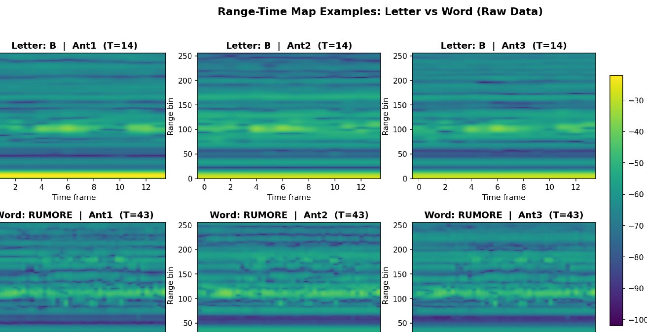
Picture a hospital room where a Deaf patient signs to a clinician, and no camera is pointed at anyone. A small 60 GHz radar measures how far the hands and arms are from the sensor, frame after frame. Nothing it records looks like a person: the output is a grid of reflected energy, with range on one axis and time on the other. The question posed by Track 2 of the CVPR 2026 Multimodal Sign Language Recognition (MSLR) challenge, part of SignEval 2026, is whether that grid carries enough information to tell 126 Italian signs apart.
Our team, AI4Good (Cristian Lazo Quispe, Universidad Nacional de Ingeniería, and Gissella Bejarano, Marist University), finished first with 0.93101 Top-1 accuracy on the private leaderboard (0.92165 public). The second-place team scored 0.91676. The method is not a new architecture. It is a recipe with three parts, which we called Mix, Measure, Merge: augmentations designed for radar spectrograms, a metric-learning term that tightens the embedding space, and a cross-validation-weighted ensemble of 83 off-the-shelf CNNs. This post walks through the reasoning, the equations, and the numbers, including the ideas that failed.
The problem
Track 2 is the radar track of a multimodal challenge. Each sample is one isolated sign from Italian Sign Language (LIS), drawn from a vocabulary of 100 medical words and 26 fingerspelled letters. Three FMCW radar antennas at 60 GHz each produce a Range-Time Map (RTM), so a sample is a tensor
$$ X \in \mathbb{R}^{3 \times T \times 256}, $$where the channel axis indexes the antenna, $T$ is the number of time frames and 256 is the number of range bins. $T$ varies from sample to sample. Letters are short (median $T = 19$ frames) and words are longer and more variable (median $T = 28$, range $14$ to $58$). The training set has 14,742 labelled clips and the test set 9,828.
The task is a standard $C$-way classification with $C = 126$: learn $f : X \mapsto \hat{y} \in \{1, \dots, C\}$. Submissions are scored by Top-1 accuracy over the $N$ held-out clips,
$$ \text{Acc} = \frac{1}{N} \sum_{i=1}^{N} \mathbb{1}\left[\hat{y}_i = y_i\right]. $$Three properties make this harder than it looks.
- The input is not a photograph. The horizontal axis is distance and the vertical axis is time. Image priors such as horizontal flips, color jitter or perspective warps have no physical meaning here.
- Letters and words are different regimes. Words involve full arm movements and produce long, rich signatures. Letters are near-static hand poses that produce brief, weak ones. In our baseline, words reached 93.0% accuracy and letters 66.1%.
- Some pairs are nearly indistinguishable at the sensor level. For M and N, the inter-class template distance on raw RTM pixels, $d = \lVert \mu_A - \mu_B \rVert^2 / \sigma^2_{\text{within}}$ (with $\mu_A, \mu_B$ the class-mean RTMs and $\sigma^2_{\text{within}}$ the within-class variance), is only 0.0055.
For context, the official SABRE baseline for this benchmark reports 81.2% accuracy.
Evaluation and validation
All experiments used stratified 5-fold cross-validation (scikit-learn StratifiedKFold, shuffled with seed 42), and the final submission was chosen from internal CV estimates rather than public leaderboard feedback.
Training 5 folds for every idea is expensive, so fold 0 served as a scout. Candidates were screened on a single deterministic fold, and only the promising ones were scaled to all five. We checked that this shortcut was safe: fold-0 rankings transferred to 5-fold CV with 14 of 15 rank positions preserved (mean $\Delta = 0.0007$).
Early stopping turned out to matter as much as any model choice. Each run tracks a moving average of validation Top-1 and stops when that smoothed curve stops improving. Raising patience from 25 to 50 epochs and setting the smoothing window to 10 reduced the inter-fold standard deviation of validation accuracy from 2.0 to 3.7 pp down to 0.2 to 0.3 pp. Without that, fold-to-fold noise would have swamped most of the effects reported below.
One practical detail of the competition format: the Kaggle submission file covers both the challenge's validation clips and its test clips. The pipeline runs inference on each split separately and concatenates the two prediction files.
The approach
Mix: spectro-temporal augmentation
The starting intuition is that every augmentation should correspond to something that can physically happen between a signer and a radar. A person signs faster or slower; a capture window starts late; the signer stands slightly closer; one antenna has a different gain. We built a taxonomy of 13 transforms around those variations, grouped by the axis they act on.
| Domain | Augmentation | Parameters | Physical motivation |
|---|---|---|---|
| Temporal | Speed-Up | $\times 1.2$ to $1.5$ | Signing speed |
| Temporal | Time Warp | $\sigma = 0.2$ | Timing variability |
| Temporal | Time Crop | ratio 0.8 to 1.0 | Partial capture |
| Temporal | Time Mask | up to 20 frames | Occlusion |
| Temporal | Temporal Shift | up to 10 frames | Alignment jitter |
| Spectral | Freq Mask | up to 20 bins | Frequency dropout |
| Spectral | Range Shift | up to 5 bins | Distance to sensor |
| Spectral | Range Zoom | $\times 0.9$ to $1.1$ | Body size |
| Spectral | dB Offset | $\pm 3$ dB | Gain variation |
| Spectral | Noise | 15 to 25 dB | Environmental noise |
| Channel | Channel Drop | $p = 0.15$ | Antenna failure |
| Channel | Channel Scale | $\times 0.8$ to $1.2$ | Gain mismatch |
| Padding | Zero Pad | to 128 frames | Length standardization |
Parameters as reported in the paper's taxonomy (Table 1).
Rather than applying a fixed pipeline, each training sample receives a random chain. Let $\mathcal{A}$ be the set of enabled transforms. We draw a chain length $n \sim \mathcal{U}\{0, 1, 2, 3\}$, sample $n$ distinct transforms $a_1, \dots, a_n$ from $\mathcal{A}$ without replacement, and apply them in sequence:
$$ \tilde{X} = a_n \circ \cdots \circ a_1 (X). $$The chain operates on the variable-length signal, before the sample is bilinearly resized to the fixed $128 \times 256$ grid the CNNs consume. So a time mask of 10 frames removes a larger fraction of a 19-frame letter than of a 43-frame word, which is the physically correct behavior.
Mixing at the batch level
On top of per-sample chains, two batch-level regularizers are applied after resizing. With probability $p_{\text{mix}}$ (0.8 in the main configurations) a batch is mixed, and when both are enabled MixUp and CutMix are chosen with equal probability, never both on the same batch.
MixUp draws $\lambda \sim \text{Beta}(\alpha, \alpha)$ with $\alpha = 0.4$, pairs each sample $i$ with a random partner $j$ from the same batch, and interpolates inputs:
$$ \tilde{x} = \lambda x_i + (1 - \lambda) x_j. $$CutMix is where the spectro-temporal structure pays off. In the released implementation, the cut is a band along the time axis that spans every range bin and every antenna. With $\lambda \sim \text{Beta}(\alpha, \alpha)$, $\alpha = 1.0$, and $T' = 128$ resized frames, a segment of length $\ell = \lfloor T'(1 - \lambda) \rfloor$ starting at a random frame $t_0$ is copied from the partner:
$$ \tilde{x}[:, t, :] = \begin{cases} x_j[:, t, :] & t_0 \le t < t_0 + \ell \\ x_i[:, t, :] & \text{otherwise.} \end{cases} $$The mixing weight is then recomputed from the actual area, $\lambda' = 1 - \ell / T'$. In both cases the loss is a convex combination of the two targets, $\lambda' \, \mathcal{L}_{\text{CE}}(\cdot, y_i) + (1 - \lambda') \, \mathcal{L}_{\text{CE}}(\cdot, y_j)$, with label smoothing applied to each term.
A pasted band forces the network to classify from a partial window of the gesture rather than any single temporal region, and every frame of the mixed sample remains a real recorded frame with all three antennas consistent. CutMix was the single largest contributor among more than 310 augmentation ablations: +2.95 pp at fold 0 when added to the chain, and 14 of the 20 best configurations in round 8 used it.
Measure: cross-entropy plus a triplet term
Mixing makes the classifier robust but does not directly ask the embedding space to separate look-alike classes such as M and N. The second pillar adds a metric-learning term. The training objective is
$$ \mathcal{L} = \mathcal{L}_{\text{CE-LS}} + \lambda_{\text{tri}} \, \mathcal{L}_{\text{triplet}}, $$where the label-smoothed cross-entropy over the predicted class probabilities $p_c$ is
$$ \mathcal{L}_{\text{CE-LS}} = -(1 - \epsilon) \log p_y - \frac{\epsilon}{C} \sum_{c=1}^{C} \log p_c, $$with $\epsilon = 0.1$ and $C = 126$, and $\lambda_{\text{tri}} \in \{0, 0.2\}$ switches between CE-only and CE + Triplet configurations.
The triplet term uses batch-hard mining on L2-normalized pre-logits embeddings $z_i$ (timm's forward_head(pre_logits=True)). With Euclidean distance $D_{ij} = \lVert z_i - z_j \rVert_2$, each anchor $i$ takes its farthest same-class sample and its nearest other-class sample in the batch:
with margin $m = 0.3$. The loss averages $\ell_i$ over anchors whose term is non-zero, and anchors without a positive in the batch are ignored. On mixed batches the triplet term uses the primary label $y_i$.
A sweep over $\lambda_{\text{tri}} \in \{0.05, 0.1, 0.2, 0.5, 1.0\}$ placed the sweet spot at 0.1 to 0.2, and it is narrow: $\lambda_{\text{tri}} = 0.3$ already degraded fold-0 accuracy.
Merge: CV-weighted probability averaging
The final prediction aggregates $C_{\text{cfg}} = 17$ training configurations. For configuration $c$ with $K_c$ completed folds and fold models $P_{c,k}$, fold softmax outputs are averaged first:
$$ \bar{P}_c(y \mid x) = \frac{1}{K_c} \sum_{k=1}^{K_c} P_{c,k}(y \mid x). $$Configurations are then combined with weights proportional to their mean cross-validation accuracy $\text{CV}_c$:
$$ P_{\text{final}}(y \mid x) = \sum_{c=1}^{C_{\text{cfg}}} w_c \, \bar{P}_c(y \mid x), \qquad w_c = \frac{\text{CV}_c}{\sum_{c'} \text{CV}_{c'}}. $$Sixteen configurations contributed all 5 folds and one (RegNetY-008) contributed 3 folds before the deadline, for $K_c \in \{3, 5\}$ and 83 models in total. Since all CV scores sit near 0.9, the weights are close to uniform; the scheme is a gentle tilt rather than an aggressive selection.
Architecture
The full pipeline, as implemented in the repository and described in the paper:
flowchart LR
    A["RTM input<br/>3 x T x 256"] --> B["Per-channel<br/>z-score"]
    B --> C["Random aug chain<br/>0-3 of 13"]
    C --> D["Resize<br/>3 x 128 x 256"]
    D --> E["CutMix / MixUp<br/>p = 0.8"]
    E --> F["5 CNN backbones<br/>4 families"]
    F --> G["CE-LS<br/>+ 0.2 Triplet"]
    G --> H["Fold average<br/>per config"]
    H --> I["CV-weighted<br/>fusion, 83 models"]
    I --> J["Top-1 class"]
The backbones are five ImageNet-pretrained architectures from four CNN families, all loaded through timm:
| Architecture | Params | Configs | Models | CV mean |
|---|---|---|---|---|
| EfficientNet-B1 | 6.7M | 10 | 50 | 0.900 |
| EfficientNet-B2 | 7.8M | 1 | 5 | 0.887 |
| ConvNeXt-Tiny | 28.6M | 2 | 10 | 0.893 |
| MobileOne-S2 | 7.8M | 2 | 10 | 0.894 |
| RegNetY-008 | 6.3M | 2 | 8 | 0.888 |
| Total | 17 | 83 |
EfficientNet-B1 is the backbone of the system, with ten configurations that vary augmentation settings, loss, epoch budget and seed. The other families exist mainly to inject diversity. The ensemble's variation comes from five sources: architecture, loss (CE vs. CE + Triplet), augmentation set (8 vs. 13 transforms, different CutMix $\alpha$), training round, and seed.
Treating the RTM as a 2D image was a deliberate choice. Temporal models (LSTMs and 1D-CNNs over the time axis) plateaued at 54% accuracy, which suggests that the range-time structure is better exploited jointly by 2D convolutions than as a sequence of independent range profiles.
Training details
All models share a common recipe, reported in the paper:
- Optimizer: AdamW, learning rate $10^{-3}$, weight decay $10^{-3}$.
- Schedule: cosine annealing over 300 epochs, 5 warmup epochs, minimum learning rate $10^{-6}$.
- Regularization: gradient-norm clipping at 1.0, dropout 0.3, drop path 0.2, label smoothing 0.1.
- Batch size: 64.
- Early stopping: patience 50 epochs on a 10-epoch moving average of validation Top-1.
- Determinism: seed 42, FP32 (no mixed precision),
torch.use_deterministic_algorithms(True),cudnn.benchmark = False.
Individual configurations deviate where a round explored something specific; the committed EfficientNet-B2 configuration (r15_b2_cm_trip), for example, uses batch size 48 and dropout 0.4. Every experiment is fully defined by its YAML file. Determinism costs speed, but across 371 experiments in 15 rounds it meant that differences between runs came from the configuration, not from GPU nondeterminism.
Results
Additive ablation
Each row adds one component to the previous configuration. Fold 0 is a single deterministic split; CV is the mean over 5 folds.
| Configuration | Fold 0 | 5-fold CV |
|---|---|---|
| CE baseline (no augmentation) | 0.8600 | n/a |
| + 8 augmentations | 0.8862 | 0.878 $\pm$ 0.01 |
| + CutMix + MixUp | 0.9078 | 0.900 $\pm$ 0.01 |
| + Triplet ($\lambda_{\text{tri}} = 0.2$) | 0.9057 | 0.915 $\pm$ 0.01 |
| 83-model ensemble, public LB | 0.92165 | |
| 83-model ensemble, private LB | 0.93101 |
Mixing is the largest single step (+4.78 pp at fold 0 over the unaugmented baseline). The triplet row is instructive: it lowers fold 0 slightly (by 0.21 pp) but raises 5-fold CV from 0.900 to 0.915, because it helps the harder folds 1 to 4 more than the already-strong fold 0. A fold-0-only evaluation would have discarded it. Going from the best single configuration (0.915 CV) to the full ensemble added a further +0.65 pp.
Which augmentations matter
Marginal fold-0 gain when each transform is added to the chain (single seed):
| Rank | Augmentation | Category | $\Delta$ Acc |
|---|---|---|---|
| 1 | CutMix ($\alpha = 1.0$) | Mixing | +2.95 pp |
| 2 | Speed-Up | Temporal | +0.82 pp |
| 3 | Time Mask | Temporal | +0.61 pp |
| 4 | Range Shift | Spectral | +0.54 pp |
| 5 | Time Crop | Temporal | +0.47 pp |
| 6 | Channel Drop | Channel | +0.38 pp |
| 7 | Range Zoom | Spectral | +0.31 pp |
| 8 | Temporal Shift | Temporal | +0.24 pp |
Two patterns stand out. CutMix contributes roughly 3.6 times more than the next transform. And the count of enabled augmentations shows a clear elbow around 8: beyond that, gains diminish and excessive distortion occasionally hurts, even though the train-validation gap keeps shrinking. CutMix $\alpha$ between 1.0 and 2.0 worked best; $\alpha = 3.0$ started to degrade accuracy.
Loss functions
EfficientNet-B1 with 13 per-sample augmentations and no batch mixing:
| Loss | Fold 0 | 5-fold CV |
|---|---|---|
| CE + label smoothing (0.1) | 0.8600 | 0.879 |
| CE + Triplet ($\lambda_{\text{tri}} = 0.1$) | 0.8952 | n/a |
| CE + Triplet ($\lambda_{\text{tri}} = 0.2$) | 0.8983 | 0.878 |
| CE + Triplet ($\lambda_{\text{tri}} = 0.3$) | 0.8633 | n/a |
| CE + SupCon ($\lambda = 0.1$) | 0.8827 | 0.881 |
| Focal loss | 0.8610 | n/a |
| ArcFace ($s = 30$, $m = 0.5$) | 0.017 | n/a |
| SphereFace | 0.018 | n/a |
One caveat, read against the additive ablation: without batch mixing, the triplet term's fold-0 gain (+3.83 pp) does not appear in 5-fold CV (0.878 vs. 0.879). Its 5-fold benefit shows up only together with CutMix and MixUp (0.900 to 0.915).
Ensemble scaling and the leaderboard
| Submission | Models | Architectures | Private LB |
|---|---|---|---|
| S9 (fold 0 only) | 10 | 1 | 0.91880 |
| S16 (4 configs) | 20 | 1 | 0.92816 |
| S15 (6 configs) | 30 | 1 | 0.92612 |
| S17 (9 configs) | 45 | 1 | 0.92897 |
| S22 (15 configs) | 75 | 4 | 0.93019 |
| S23 (17 configs) | 83 | 5 | 0.93101 |
| 2nd place | 0.91676 |
A 20-model ensemble of four EfficientNet-B1 configurations (S16) already reaches 0.92816, 1.14 pp above second place. The training recipe, not ensemble size, is the primary source of the margin. Adding three more CNN families on top takes the private score from 0.92816 to 0.93101; the paper attributes about +0.22 pp cumulatively to the new families alone. Note also that more models of the same family is not monotonic: S15, with 30 models, scored below S16, with 20.
A subset analysis (100 random subsets per ensemble size, drawn from the 17 configurations) shows diminishing returns: agreement with the full ensemble's predictions is 95% at $k = 2$ and 99% at $k = 12$.
The final margin over second place was 1.43 pp, in a field of 13 teams and 27 submissions. The private score was 0.94 pp higher than the public one, consistent with a CV protocol that did not overfit the public split.
Where the errors live
Most remaining error is in letters: words average 93.0% accuracy, letters 66.1%, with U (40.3%), D (42.1%) and E (43.6%) the worst. Silhouette scores agree (0.501 for words, 0.137 for letters). The confusable pairs M/N, U/V, D/O and E/F all have $d < 0.01$, which points to a sensor-level limitation at 60 GHz rather than a modeling failure. A per-sample oracle over ensemble members would reach 0.9891, an upper bound on what learned routing could recover.
What did not work
All of the following are documented in the paper:
- Angular-margin losses collapsed. ArcFace ($s = 30$, $m = 0.5$) and SphereFace reached 0.017 and 0.018 Top-1, close to chance for 126 classes. Our interpretation is that radar signatures of a single sign vary too much for the tight hyperspherical clusters these losses enforce.
- Supervised contrastive loss reached a competitive 0.883 and added diversity, but was consistently dominated by CE + Triplet.
- Focal loss was indistinguishable from the CE baseline at fold 0 (0.8610 vs. 0.8600).
- Temporal models (LSTMs and 1D-CNNs on the time axis) plateaued at 54%.
- Stacking and confidence gating on out-of-fold predictions overfit and were not adopted; plain CV-weighted averaging won.
- More augmentation past roughly 8 transforms, CutMix $\alpha = 3.0$, and $\lambda_{\text{tri}} = 0.3$ all degraded results.
Lessons
- Design augmentations from the sensor, not from ImageNet. The most useful transforms (speed changes, time masks, range shifts, channel drops) each mirror a real source of variation in radar capture.
- Check all folds before discarding an idea. The triplet term lowered fold 0 and raised 5-fold CV by 1.5 pp. Single-fold scouting ranks well, but misses effects that live in the harder folds.
- Regularizers interact. The triplet loss alone did not move 5-fold CV; combined with mixing it did.
- Diversity beats repetition. More EfficientNet-B1 configurations gave non-monotonic returns; new families added a steady gain, and about 12 configurations capture most of the ensemble's benefit.
- Determinism is a research tool. Bit-identical runs and smoothed early stopping (fold std of 0.2 to 0.3 pp) made 371 experiments comparable at the resolution of tenths of a point.
Reproducibility
Everything is public under the MIT license at CristianLazoQuispe/CVPR-SignEval2026:
codes/final/train.pyis one deterministic training script for all loss modes; every experiment is a YAML file underconfigs/(rounds 9 and 12 to 15 form the final ensemble;configs/ablation/holds the augmentation ablations).scripts/build_s23.shrebuilds the winning S23 submission end to end: inference, CV-weighted fusion, and joining the validation and test prediction files.- All 83 S23 checkpoints (about 2.9 GB) are on the Hugging Face Hub at
CristianLazoQuispe/CVPR-SignEval2026-models, so the ensemble can be rebuilt without retraining. codes/final/validate_reproducibility.pychecks bit-identical reruns, which hold under identical hardware and software.
The paper appears in the CVPR 2026 Workshops proceedings (pages 10528 to 10537), and the poster was presented in person at CVPR 2026 in Denver.