Robustness is the blind spot of deepfake detection: standard detectors collapse to roughly 0.5 AUC, chance level, once images are even mildly blurred, re-compressed, or downscaled. That is what happens to a face photo after a cheap camera and a couple of messaging apps, and exactly what someone hiding a manipulation would do on purpose. The NTIRE 2026 Robust Deepfake Detection Challenge, held at CVPR 2026 and organized by Benedikt Hopf and Radu Timofte, was built around this failure mode: classify face images as real or fake when the test images carry degradations, and generators, that the training set never shows you.
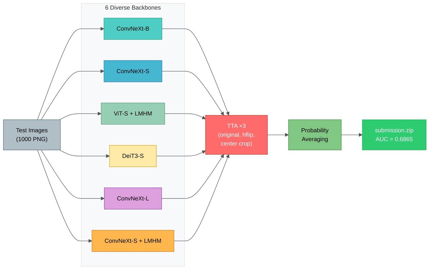
My solution, submitted as team AI4Good / SoloUNI, rests on a counter-intuitive decision. The final models never see a single real deepfake during training. They are trained on the 500 real images of the training set alone. Fakes are synthesized on the fly by blending one real face into another along facial landmarks (Self-Blended Images), and every sample, real or synthetic, is passed through the PMM degradation model before it reaches the network. Six backbones trained this way are averaged with test-time augmentation. The ensemble reaches 0.7777 AUC on a local hard test and 0.6865 AUC on the CodaBench public test, and the method is described in Section 3.12 of the official challenge report.
This post covers why that decision was necessary, how the pipeline works, how I validated it with almost no leaderboard feedback, and what failed.
The problem
Each sample is an RGB face image $x \in \mathbb{R}^{H \times W \times 3}$ with label $y \in \{0, 1\}$, where $y = 0$ means real and $y = 1$ means fake. The goal is a scoring function $s : x \mapsto [0, 1]$ that estimates $P(y = 1 \mid x)$. The submission is one probability per test image, in alphabetical filename order.
The data is tiny. The labelled training set has 1,000 PNG images at $256 \times 256$, perfectly balanced at 500 real and 500 fake. A 100-image unlabelled validation set was scored on CodaBench during the development phase, and the public test set has 1,000 images. According to the challenge description, each split uses different base identities and different generative methods, and the validation and test splits carry additional degradations not present in training. The public test phase allowed a single submission.
Submissions are ranked by the area under the ROC curve. With $\mathcal{P}$ the set of fake test images, $\mathcal{N}$ the set of real ones, and $s_i$ the score of image $i$, the AUC is the probability that a randomly chosen fake is scored above a randomly chosen real:
$$ \text{AUC} = \frac{1}{|\mathcal{P}|\,|\mathcal{N}|} \sum_{i \in \mathcal{P}} \sum_{j \in \mathcal{N}} \left( \mathbb{1}\left[s_i > s_j\right] + \tfrac{1}{2}\,\mathbb{1}\left[s_i = s_j\right] \right). $$AUC depends only on the ranking of the scores, not their calibration, so no threshold needs tuning.
The difficulty compounds: 1,000 images invite a supervised model to memorize whatever separates these particular fakes from these particular reals, the test generators are unseen so such memorization is useless, and the degradations destroy the high-frequency traces many detectors rely on.
Evaluation and validation
With limited validation-phase submissions and a single public-test shot, the central engineering problem was a local metric that predicts the leaderboard. The obvious choices do not.
My first models were trained in the standard supervised way on the labelled real and fake images. The table below, reconstructed from the experiment log in the repository history, compares each local validation scheme with the CodaBench validation AUC of the corresponding submission.
| Local validation scheme | Local AUC | CodaBench AUC | Gap |
|---|---|---|---|
| Stratified K-fold on labelled images (CLIP ViT-B/16) | 0.89 | 0.66 | 0.23 |
| 50/50 holdout of the labelled images (CLIP ViT-L/14, frozen) | 0.90 | 0.65 | 0.25 |
| Leave-one-source-out, 7 folds (ConvNeXt-Tiny) | 0.84 | 0.67 | 0.17 |
| Leave-one-source-out with PMM degradation | 0.80 | 0.65 | 0.15 |
| Hard test, SBI-trained ensemble | 0.779 | 0.71 | 0.069 |
Stratified folds and random holdouts were nearly useless: both halves come from the same identities and generators, so they reward memorization. Leave-one-source-out (LOSO) cross-validation, where folds are defined by image source categories that I derived from Gemini annotations of every training image (movie still, TV show, webcam, surveillance, and so on), shrank the gap from 0.23 to 0.17. Still, every CodaBench score in this period clustered between 0.65 and 0.67 regardless of backbone or recipe.
Adversarial validation pointed to the reason. A classifier trained to separate training images from validation images, on hand-crafted pixel statistics or on CLIP embeddings, did no better than chance (AUC 0.50 and 0.54). On the public test set the picture changed: color and degradation features separated training images from test images with an adversarial AUC of 1.0, with the test set noticeably less saturated and smoother (fewer edges, less high-frequency energy, fewer JPEG block artifacts). Gemini annotations of a sample of test images described blur in 82% of them and noise in 70%.
The local metric that finally worked is the hard test. It takes the 1,000 labelled images and applies the PMM degradation model to each at a higher strength than used in training (strength 0.7, per-operation probability 0.5). Once the models are trained only on reals, the 500 labelled fakes become something precious: fakes from a generator the model has never seen, under degradations, which is a reasonable miniature of the test condition. Its gap to CodaBench was 0.069, a third of the LOSO gap, which made offline iteration possible. All per-model numbers in this post refer to this set.
Two caveats. The 500 reals in the hard test are the training reals under fresh, stronger degradations, so the real side of the ROC curve is easier than it would be on new identities. And because the ensemble was chosen by greedy selection on the hard test, its hard-test AUC is an optimistic, in-sample estimate. The public test result (0.6865) sits 0.09 below the ensemble's hard-test value (0.7777), consistent with both. A second hard test (v2), whose degradation probabilities were matched to the measured test profile, was used as a cross-check.
The approach
The key idea comes from Self-Blended Images (SBI, Shiohara and Yamasaki, CVPR 2022) and from the organizers' own PMM work (Hopf and Timofte): rather than learning what a particular generator's output looks like, teach the model what a blended face looks like. Many face manipulations, whatever produced the new content, end by pasting a synthesized region back into a real frame. That step leaves boundary, color, and texture inconsistencies that are largely independent of the generator. If the model can only learn those inconsistencies, because they are the only thing separating its two classes, it has nothing generator-specific to memorize.
Concretely, for a target real image $x_t$, a donor image $x_d$, and a soft mask $M \in [0,1]^{H \times W}$ derived from the target's facial landmarks, the alpha-blended pseudo-fake is
$$ \tilde{x} = r\,M \odot T(x_d) + \left(1 - r\,M\right) \odot x_t , $$where $\odot$ is element-wise multiplication (the mask is broadcast over the color channels), $T(\cdot)$ is a random source transformation followed by color matching to $x_t$, and $r \in [0.05, 1]$ is a blend ratio that controls how visible the pasted region is. The pseudo-fake gets label $y = 1$ and the untouched $x_t$ keeps $y = 0$.
The details, as implemented in src/data/sbi_proper.py:
- Donor. The original SBI blends an image with a transformed copy of itself. The variant used in the final models (
cross_blend) draws the donor from another real image of the training pool, resized to the target. - Source transform $T$. Random color jitter, RGB shift, Gaussian blur, downscale-upscale (a resolution mismatch), and horizontal flip, each with its own probability. With probability 0.7 the donor's per-channel mean and standard deviation are then matched to the target's.
- Mask $M$. 68-point landmarks from
face_alignment(FAN), pre-extracted for the training images. Each sample draws one of four mask types: the convex hull of the jaw line, a single face part (an eye, the nose, a cheek, a lip, and so on), the hull of 4 to 15 random landmarks, or the hull of all 68 points. The mask is Gaussian-blurred twice, with a second kernel drawn from $[11, 71)$, so the blending boundary ranges from sharp to very soft. - Blend ratio $r$. With probability 0.3 the sample is a deliberately subtle "hard negative" with $r \sim \mathcal{U}(0.05, 0.20)$; otherwise $r \sim \mathcal{U}(0.05, 1.0)$.
- Blending operator. Half the time the formula above is used. The other half uses Poisson (gradient-domain) blending via OpenCV's seamless cloning, which pastes the donor's gradients inside the mask while matching the target's pixels on its boundary. This removes the visible seam.
Each training sample is a pseudo-fake with probability 0.5 and a real otherwise.
Degradation is applied to both classes. After blending, every sample, real or pseudo-fake, passes through the PMM degradation function with probability 0.4 and strength 0.3. The implementation is adapted from the BSRGAN degradation code: a randomly shuffled sequence of up to 13 operations (smoothing, resizing, Gaussian, Poisson and speckle noise, enhancement, JPEG, sharpening), each applied with probability 0.5 except the rarer noise types, followed by a final JPEG compression and a resize back to the input size. Because degradation is independent of the label, the model cannot use it as a shortcut and must find blending evidence that survives it. On top of PMM, a standard Albumentations pipeline adds blur, noise or JPEG, downscaling, and brightness and contrast changes.
Architecture
The six ensemble members share one pipeline and differ in backbone, seed, batch size and patience, and in whether a fourth input channel carries a landmark heatmap.
flowchart LR
  subgraph TRAIN["Training (per model)"]
    R["500 real faces"] --> C{"p = 0.5"}
    C -->|"real, y=0"| PMM
    C -->|"fake, y=1"| SBI["SBI blend<br/>Poisson or alpha"]
    LM["FAN 68 landmarks"] --> MASK["Landmark mask"] --> SBI
    D["Donor real"] --> TR["Source transform<br/>+ color match"] --> SBI
    SBI --> PMM["PMM degradation<br/>p=0.4, s=0.3"]
    PMM --> AUG["Albumentations<br/>224x224"]
    AUG --> HM["+ heatmap channel<br/>LMHM only"]
    HM --> NET["timm backbone<br/>+ BN-linear head"]
    NET --> LOSS["BCE with<br/>label smoothing"]
  end
  subgraph INFER["Inference"]
    X["Test image"] --> TTA["3 TTA views"]
    TTA --> M6["6 models"]
    M6 --> AVG["Mean of sigmoids"]
    AVG --> S["P(fake)"]
  end
  NET -.->|"best.pt"| M6
Each model is a timm backbone with its classification head removed, followed by a BatchNorm1d and a single linear layer that outputs one logit. The backbones are ConvNeXt-Small, -Base and -Large (ImageNet-22k pretrained, fine-tuned on ImageNet-1k), DeiT3-Small, and ViT-Small. Together they span 22M to 197M parameters.
Two of the six models (lmhm_css and lmhm_vits) take a 4-channel input: the RGB image plus a heatmap rendered from the 68 landmarks, each point drawn as a Gaussian with $\sigma = 4$ pixels at $224 \times 224$ and rescaled to $[-1, 1]$. The heatmap gives the network an explicit prior on where face parts are, which is where the blending masks live.
Training details
All six models are trained independently with the same recipe. The values below are taken from the shipped YAML configurations, which the checkpoints also embed.
| Setting | Value |
|---|---|
| Input | $224 \times 224$, ImageNet normalization |
| Training data | 500 real images only (cv_mode: sbi_proper) |
| SBI | pseudo-fake probability 0.5, Poisson probability 0.5 |
| PMM | probability 0.4, strength 0.3 |
| Augmentation | Albumentations "moderate" preset |
| Optimizer | AdamW, lr $3 \times 10^{-5}$, weight decay 0.05 |
| Schedule | 1 linear warm-up epoch, then cosine annealing |
| Epochs | up to 100; early-stopping patience 25 (10 for r3e_fa_css) |
| Batch size | 8 (ConvNeXt-Base, ConvNeXt-Large) or 16 (others) |
| Loss | binary cross-entropy, label smoothing 0.05 |
| Regularization | gradient clipping at 1.0; dropout and drop-path 0 |
| Precision | FP32, deterministic algorithms, fixed seeds (42; 43 for ConvNeXt-Large) |
With label smoothing $\varepsilon = 0.05$, the target for a sample with label $y$ becomes $y' = (1 - \varepsilon)\,y + \varepsilon/2$, and the loss for a logit $z$ is
$$ \mathcal{L}(z, y') = -\,y' \log \sigma(z) - (1 - y') \log\left(1 - \sigma(z)\right), $$where $\sigma$ is the logistic sigmoid. Smoothing keeps the logits from growing without bound on a pseudo-fake task that the network can eventually solve almost perfectly.
Checkpoints are selected on a validation set built like the training set: the same 500 reals with an independent stream of pseudo-fakes, without PMM or augmentation. Each run trains a single fold, and the pipeline is deterministic (torch.use_deterministic_algorithms, seeded workers, AMP disabled).
Ensemble and test-time augmentation
At inference, each image is resized to $224 \times 224$ and presented to every model under $T = 3$ views: the original, a horizontal flip, and a mild brightness and contrast perturbation (limits of $\pm 0.1$, with a fixed seed). With $f_m$ the logit of model $m$, $\tau_t$ the $t$-th view, and $M = 6$ models, the submitted score is a plain average of probabilities:
$$ s(x) = \frac{1}{M} \sum_{m=1}^{M} \frac{1}{T} \sum_{t=1}^{T} \sigma\!\left( f_m\!\left( \tau_t(x) \right) \right). $$The six members were chosen by greedy forward selection on the hard test: starting from an empty set, repeatedly add the candidate that most increases ensemble AUC, and stop when nothing helps. The selection script also implements rank and AUC-weighted averaging; the submission uses the plain probability average above.
Results
Per-model and ensemble AUC on the local hard test (500 real and 500 fake images, PMM-degraded):
| Model | Backbone | Input | Hard-test AUC |
|---|---|---|---|
r3d_fa_csb |
ConvNeXt-Base | RGB | 0.7644 |
lmhm_css |
ConvNeXt-Small | RGB + landmark heatmap | 0.7268 |
r3e_fa_css |
ConvNeXt-Small | RGB | 0.7259 |
r3d_fa_csl_s43 |
ConvNeXt-Large (seed 43) | RGB | 0.7127 |
r3d_fa_deit3_s |
DeiT3-Small | RGB | 0.7111 |
lmhm_vits |
ViT-Small | RGB + landmark heatmap | 0.6945 |
| Ensemble (6) + TTA | 0.7777 |
On CodaBench, this ensemble scored 0.6865 AUC on the public test (submission 632762). In the validation phase, the first SBI-trained ensemble raised the CodaBench validation AUC from the 0.65 to 0.67 plateau of all supervised approaches to 0.71.
The ensemble beats its best member by 0.013, a modest gain since all members share one recipe and differ mostly in inductive bias. ConvNeXt variants dominate, and the weakest model, lmhm_vits, still made the greedy cut: it contributes diversity rather than accuracy.
What did not work
The repository history keeps an experiment map with every round's numbers. The negative results are as informative as the final recipe.
Supervised training on the labelled fakes. Every model trained on real and fake labels landed between 0.65 and 0.67 on CodaBench validation, and ensembling two of them stayed at 0.66.
External data. Pretraining on external face-forgery data (DFF and DF40) and fine-tuning on the competition data gained 0.007 on the local holdout (0.835 vs. 0.828). A frozen CLIP ViT-L/14 with a pretrained head reached 0.903 on the local 50/50 holdout and only 0.65 on CodaBench.
PMM degradation without SBI. Adding PMM to the supervised LOSO pipeline lowered LOSO AUC from 0.84 to 0.80 and CodaBench from 0.67 to 0.65. Degradation alone does not fix a model that has learned the wrong features.
Stronger or test-matched degradation. A "test-profile" variant with PMM probability 0.8, strength 0.4 and a targeted hue and saturation shift scored 0.7079 on the hard test with ConvNeXt-Small, against 0.7259 for the standard setting. The project notes record that strength 0.3 also beat 0.0, 0.5 and 0.7.
Color augmentation. HSV augmentation, the obvious response to the measured color shift, hurt: 0.656 on the hard test for ConvNeXt-Small, and a variant combining aggressive color shifts, RTMPose landmarks and external donors was worse than the plain recipe on every metric.
Better landmark detectors. RTMPose detected a face in 100% of images on every split, against roughly 95% for face_alignment and 76% to 80% for MediaPipe. Yet for the same backbone and seed, models built on RTMPose masks scored lower on the hard test (for example, 0.6628 vs. 0.7127 for ConvNeXt-Large with seed 43).
Harder pseudo-fakes. An "SBI Hard Mode" variant, which drew donors from an external pool of real faces and used subtler blends, lowered the SBI validation AUC, as intended, but also lowered the hard-test AUC (0.693 vs. 0.778 for ConvNeXt-Large). JPEG re-encoding as a proxy for generator artifacts also hurt (0.661 vs. 0.728 in a pretraining run).
Some backbones. Under the same SBI recipe, ResNet-50 stayed at chance (about 0.49 to 0.50), EfficientNet-B3 reached 0.540, and Swin-Tiny 0.657 to 0.668. ViT-B models initialized from deepfake-pretrained Hugging Face checkpoints stayed well below the ConvNeXt models (0.629 to 0.682).
Lessons
Validate on the shift you expect, not on the data you have. Random folds of the labelled data were off by 0.23 AUC; a holdout of unseen fakes under degradation was off by 0.069. When the test distribution differs by construction, validation design matters more than the model.
When the generators change, remove the generator from training. Training only on reals with synthetic blends broke a plateau that no supervised variant, external dataset, or backbone change could move. Not seeing the labelled fakes is what turned them into a usable test set.
An in-distribution synthetic validation set is not a proxy. ConvNeXt-Small, ConvNeXt-Large, ViT-Small and EfficientNet-B3 all scored between 0.982 and 0.999 on SBI validation, yet their hard-test AUCs ranged from 0.540 to 0.778. The pseudo-fake task is easy to solve; what matters is whether the solution transfers.
More realism in augmentation is not monotonically better. Stronger degradations, test-matched color shifts, harder pseudo-fakes and a landmark detector with perfect coverage each looked like improvements on paper and each lowered hard-test AUC.
Seeds and selection noise are large at this data size. The same configuration with seed 42 vs. 43 differed by 3% to 7% in hard-test AUC. With 1,000 evaluation images, small differences between single runs should not drive decisions, and ensemble scores selected on the same set should be read as upper bounds.
Reproducibility
The repository contains the six configurations, the training and inference code, and the factsheet. All six checkpoints (about 1.6 GB) are on the Hugging Face Hub, and each best.pt embeds its training configuration.
cp .env.example .env          # set DATA_ROOT (data and experiments live outside the repo)
pip install -r requirements.txt

# Pretrained checkpoints into $DATA_ROOT/experiments/<model>/best.pt
pip install -U "huggingface_hub[hf_transfer]"
HF_HUB_ENABLE_HF_TRANSFER=1 hf download CristianLazoQuispe/RobustDeepfakeCVPR26-models \
  --repo-type model --local-dir "$DATA_ROOT/experiments"
# move each to <model>/fold0/best.pt for inference

# Train one model
python codes/train.py configs/round3d_diversity/r3d_fa_csb.yaml --device cuda:0

# 6-model ensemble inference with TTA, packaged for CodaBench
python scripts/ensemble/generate_ensemble_submission.py \
    --models r3d_fa_csb r3e_fa_css lmhm_vits r3d_fa_deit3_s r3d_fa_csl_s43 lmhm_css \
    --device cuda:0 --tta --output greedy6_final.zip
Greedy ensemble selection lives in scripts/ensemble/greedy_ensemble.py, and the hard test is generated by scripts/data/create_hard_test.py. Training used NVIDIA A100 GPUs, used no extra data, and each model trains on a single fold. The factsheet's short summary lists a learning rate of $10^{-4}$ and patience 10; the YAML files above, which the released checkpoints embed, are the authoritative values.
The factsheet lists three open directions: pretraining on large face-forgery datasets before SBI fine-tuning, diffusion- or GAN-based pseudo-fakes instead of blending, and training all five folds per backbone. The broader lesson for any detection problem with a moving target is simpler: decide what the test will differ in, build a small local set that differs in the same way, and let that set decide what goes into the model.