Day 1 of DL4SCI 2026 was, almost entirely, a day about generative models: what they are good for in science, and why they are still too slow. The morning moved from motivation to mechanism. Arash Vahdat argued that scientific data breaks the assumptions vision models were built on, and that a surprising amount of scientific design can be rewritten as sampling from a reward-tilted distribution. Julius Berner then took the sampling machinery apart piece by piece, from architecture and latent spaces down to the geometry of the generative trajectory and the distillation tricks that compress hundreds of solver steps into a handful. The afternoon turned to applications: a proposal to treat physics itself as a foundation-model problem, and a short talk on atomic foundation models for science. The thread running through the whole day is that in science the interesting part of the distribution is usually the part a model fits worst.
Talks
Generative AI for Science — Arash Vahdat (Nvidia)
Vahdat opened with the gap between generative modeling as the vision community practices it and generative modeling as science needs it. His framing: the tooling transfers, the assumptions do not, and the failure modes that matter in science live in the tails of the distribution rather than near its mean. He then walked through design as a generative problem, with molecules and proteins as the concrete cases.
He also gets credit for the best line of the day: he joked that his cat is more famous than he is, since he uses it so often as the example image when illustrating the diffusion forward process.
Weather is not a natural image
Modeling weather with a generative vision model looks superficially like generating video. Vahdat's point was that it is very different in three specific ways.
- The data has a different character. These are physical fields, not photographs, and the inductive biases that make natural images easy do not obviously apply.
- Each variable has its own dynamic range. Temperature, pressure, wind and humidity live on different scales, so a single normalization scheme treats them unequally.
- The channels are correlated physically, not perceptually. The relationship between temperature and pressure channels is constrained by physics, unlike the loose statistical coupling between the R, G and B channels of a photograph.
The tails are the product
The second half of the motivation was about extreme events. Reliable forecasting of extreme weather requires a generative model that places mass correctly on rare, high-impact points: temperature spikes, heat waves, outliers. Most days are boring, with values close to the norm, and a model trained to minimize an average loss will happily be excellent at boring days. The cases that matter operationally are precisely the uncommon ones. So the evaluation question becomes tail fidelity rather than average fidelity, and that is the part current models fit worst.
Design as sampling from a tilted distribution
Vahdat then reframed scientific design. The naive statement of the problem is a constrained maximization,
$$\max_{x \in F} R(x; c)$$
where $x$ is a candidate design, $F$ is the feasible set (valid molecules, designable proteins), and $R(x; c)$ is a reward function conditioned on some context $c$. The difficulty is that $F$ has no tractable description: nobody can write down the set of synthesizable molecules as constraints.
The generative move is to replace feasibility by likelihood. Train $p_\theta(x)$ on a corpus of valid molecules or designable proteins, and treat membership in $F$ as being a plausible sample from that model: staying on the data manifold is what it means to be feasible. The constrained maximization then becomes sampling from an optimal reweighted distribution,
$$q^*(x) \;\propto\; p_\theta(x)\,\exp\!\big(R(x; c)/\lambda\big)$$
where $\lambda > 0$ is a temperature. Small $\lambda$ sharpens $q^*$ toward high-reward designs at the cost of drifting from the prior; large $\lambda$ keeps the samples close to $p_\theta$ and therefore close to things that plausibly exist. The exponential tilt is the standard way of trading reward against staying in distribution.
Three paradigms attack that target distribution, and they differ mainly in when the compute is spent.
| Paradigm | What it changes | When |
|---|---|---|
| Generative training | Learns $p_\theta(x)$ from valid data | Training time |
| Post-training alignment with RL | Fine-tunes weights toward $R$ | After pre-training |
| Test-time search | Guides or searches at sampling time | Inference, no weight updates |
Molecules: representation and generation order
For small molecules the representation choice matters as much as the model. Vahdat contrasted two string encodings: SMILES, the standard linear notation for a molecule, and SAFE (Sequential Attachment-based Fragment Embedding), a fragment-based string representation designed so that generation can proceed at the level of chemical fragments rather than individual atoms.
On top of SAFE he presented GenMol, a fragment-based discrete diffusion model. The interesting property is the generation order: GenMol can fill in tokens in arbitrary order, whereas an autoregressive model such as SAFE-GPT must emit them sequentially, one after another in a fixed direction. For molecular design that flexibility is natural, since a chemist's constraints rarely arrive in left-to-right order; one often wants to fix a scaffold and generate around it.
The fourth topic of the talk was synthesizability. A generative model can produce a molecule that scores well and still be useless if no one can make it. ReaSyn (Reaction Synthesis) improves synthesizability projection: an encoder-decoder transformer that autoregressively predicts the synthetic pathway, the sequence of reactions, for a given target molecule. Predicting the route is what turns a proposal into something a lab can act on.
Proteins: La-Proteina and Complexa
Topic five was La-Proteina, a model for fully atomistic protein design, which Vahdat presented as a genuinely hard problem: committing to every atom's position is much more demanding than producing a coarse backbone. The architecture he showed is an encoder-decoder.
Topic six was binder design, with Complexa as the approach. A binder is a designed protein that must attach to a specific target, another protein, a receptor or an antigen, with high affinity and high specificity. The difficulty is the interface: the geometry and chemistry of the contacting atoms have to be right, and the rest of the molecule has to hold that interface in place. Vahdat also described a large-scale wet-lab validation campaign, in which many designed binders were synthesized and experimentally tested rather than only scored in silico. In a field where generative metrics are easy to game, that is the only evidence that counts.
Background primer: structure prediction is not binder design
Background primer: written after the school from general knowledge, not part of the speaker's slides.
Two problems are easy to confuse. Structure prediction asks: given this amino-acid sequence, what shape does it fold into? It is fundamental because a protein's function follows from its shape, and it is general purpose, useful for understanding disease, enzymes and small-molecule drugs alike. Binder design is the inverse problem: given a target, invent a sequence and structure that sticks to it. The second builds on the first, because you need the target's three-dimensional shape before you can design anything to attach to it.
It is also worth remembering that a predicted structure is one representative conformation, like a single photograph. A real protein fluctuates and exists as an ensemble, and on an induced-fit view both binder and target can adjust shape to fit each other, so the lock-and-key picture is an approximation. Dynamics refines the base prediction rather than replacing it: the protein fluctuates around the predicted structure, it does not jump to arbitrary shapes.
Why design new binders at all? Nature has not supplied a binder for every target of interest, and screening enormous libraries in the lab is slow and expensive. A generative model that proposes a custom binder for a named target is an attempt to shortcut that search, which is exactly why the wet-lab hit rate is the metric that matters.
Q&A
One question challenged the distributional choice directly: a t-distribution may not be adequate for capturing the tails, the extreme and rare events. Vahdat acknowledged the point and said it is ongoing work. That closes the loop with the opening motivation. The hardest part of generative modeling for science is not generating a plausible average sample, it is getting the rare ones right.
Accelerated Diffusion Models — Julius Berner (Nvidia)
Berner's talk had one organizing complaint: diffusion and flow models produce impressive results, and video diffusion models take several minutes to generate a short clip. Everything else was a taxonomy of the ways to pay less for the same sample, ordered roughly from architecture to trajectory geometry to distillation.
Flow and diffusion models in one page
The flow-matching view needs three ingredients. An interpolation defines a path $x_t$ between data and noise, in the simplest case the linear interpolation
$$x_t = (1 - t)\,x_0 + t\,x_1$$
with $t \in [0,1]$ the interpolation time, $x_0$ the noise endpoint and $x_1$ the data endpoint. A velocity field $v_\theta(x_t, t)$, the learned object, tells each point which direction to move and how fast. Generation is then integration: start from noise and follow the velocity field by numerically solving the associated ordinary differential equation, which in practice means taking a sequence of discrete steps, each one evaluating the network once. The number of those evaluations is the cost of a sample, and almost every acceleration method in the talk is an attack on that number or on the cost per evaluation.
Architecture and dimensionality
The prevalent architecture is the Diffusion Transformer (DiT) applied to non-overlapping image patches as tokens, with adaptive layer normalization (adaLN) carrying the time conditioning. The benefit is strong performance and clean scaling. The cost is that attention scales quadratically in the number of tokens, and the token count grows rapidly with resolution, so high-resolution images and long videos become expensive fast.
Two responses follow. The first is dimensionality reduction: latent diffusion maps the data into a compressed latent space, for instance with a VAE, and runs the diffusion process there. Fewer tokens means a direct cut in the quadratic term. The second is efficient architectures that exploit the structure of attention itself. Berner noted that attention scores typically show high sparsity, with the caveat that the sparsity pattern is conditioned on the model and depends on the layer and head, so it is not a free structural assumption. Sub-quadratic options include sparse, local and linear attention, and state-space models; hybrid architectures pair global attention with convolutional layers that handle local structure.
Underneath all of this sits general systems work that applies to any model: hardware optimization through kernel fusion, graph compilation and FlashAttention, and precision reduction through quantization of weights and activations. He used FLUX.2-dev inference as a case study of these applied together.
Better solvers, better trajectories
Improving the numerical solver is the most direct lever on step count. The available knobs are adaptivity, solver order, use of history, and reparametrizations, plus the choice of time discretization, which can be adaptive or learned rather than a fixed uniform grid.
Trajectory design is the more interesting lever: instead of integrating a hard path more cleverly, reshape the path so that it is easy to integrate. Three ingredients influence the ODE trajectories.
- The data or prior distribution. Here the goal is a latent space with better diffusibility, for example replacing the VAE with a representation encoder whose latent is straighter to diffuse through.
- The coupling, meaning how noise is paired with data during training. Options include mini-batch optimal transport, which re-pairs samples within a batch, using a pre-trained flow through reflow or rectified flow, or learning the conditional $p(x_t \mid x_0)$ outright.
- The interpolant, which can be made learnable and trained with a straightness objective, so that paths are as close to straight lines as possible and therefore need fewer steps.
Background primer: why coupling diagrams have crossing lines
Background primer: written after the school from general knowledge, not part of the speaker's slides.
The coupling slide is worth unpacking, because the picture explains the whole idea. Put starting points $x_0$ drawn from the noise prior on the left and data points on the right, and draw a line for every training pair.
With independent coupling, each noise sample is paired with a randomly chosen data point. A noise point near the top of the prior may be paired with a data point near the bottom, and vice versa, so the lines cross. Crossings are the problem: the model learns a single velocity $v(x,t)$ per point and time, so wherever two training trajectories cross it must average conflicting directions. The resulting marginal field is curved, and a curved field needs many small steps to integrate accurately.
With optimal-transport or reflow coupling, the pairs are rearranged so that the lines do not cross. Reflow, or rectified flow, does this empirically: train a first flow, use it to transport noise to data, re-pair each noise sample with the data point it actually flowed to, and retrain. Iterating straightens the trajectories until they can be integrated in very few steps, sometimes close to one.
Two clarifications are worth stating explicitly. First, the two blobs drawn on each side are about modes, not errors. On the data side they are two modes of a multi-modal data distribution, cats and dogs in the usual cartoon; on the noise side the prior is a single Gaussian, drawn as two sub-groups only to track which noise regions get routed to which mode. Second, crossing does not produce wrong samples: both couplings learn the correct distribution, and with enough steps both generate valid samples from every mode. Crossing is a speed problem, nothing more.
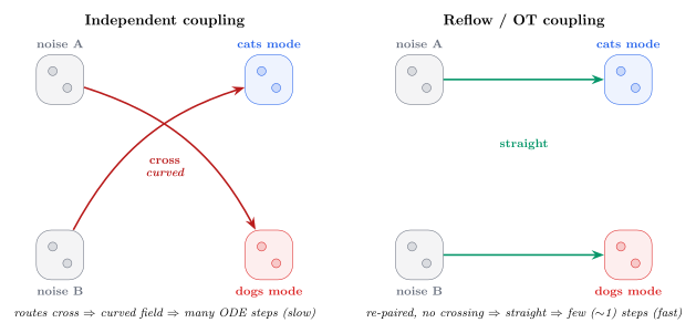
Figure: on the left, independent coupling routes noise to data along crossing lines, giving a curved velocity field that needs many ODE steps; on the right, reflow or optimal-transport coupling re-pairs the samples so the routes do not cross, yielding straight paths integrable in very few steps.
Step distillation
The other route to few-step sampling is to distill a slow many-step teacher into a fast few-step student, matching either the teacher's trajectory or its distribution. Berner used a single parametrization throughout,
$$f_{s,t}(x_s) = x_s + (t - s)\,v_{s,t}(x_s)$$
where $f_{s,t}$ is the flow map taking a state at time $s$ to time $t$, and $v_{s,t}$ is a learned average velocity initialized from the teacher. The form is inspired by mean velocity, and more general parametrizations exist. The boundary condition $f_{t,t}(x_t) = x_t$, that a zero-length jump does nothing, matters for several of the methods.
Progressive distillation learns large jumps from smaller ones: a student learns to take one step that matches two teacher steps, and repeating the procedure halves the step count each round. It is cheap, on the order of three forward passes, and needs no full trajectory. The costs are compounding errors across rounds, plus either multiple iterations when using a frozen map, or a moving target in the loss together with an extra loss at $t = s$ enforcing the identity when not.
Consistency models and Eulerian flow maps instead enforce consistent predictions along a trajectory: every point on a path should map to the same target. The objective involves the derivative of the flow map with respect to the source time,
$$\left\lVert \frac{d}{ds} f_{s,t}(x_s) \right\rVert$$
which penalizes how much the prediction changes as $s$ moves. Under perfect self-consistency this quantity stays near zero along the trajectory. This is the Eulerian or differential view, differentiating with respect to where the jump starts.
Lagrangian flow maps take the complementary view, tracking the particle along its trajectory. Differentiating $f_{s,t}(x_s) = x_t$ with respect to the target time $t$ instead of $s$ gives
$$\frac{d}{dt}\, f_{s,t}(x_s) = v_t(x_t)$$
so moving the target time makes the map's output move with the velocity field evaluated at the endpoint. The constraint is on the arrival rather than the departure.
Adversarial distillation uses projected GANs on teacher features with diffusion initialization: the adversarial loss is computed on projected features taken from the teacher, and the student starts from the pretrained diffusion weights.
Variational score distillation computes a divergence using the teacher score. The student is matched to the teacher through a divergence whose gradient is expressed via the teacher's score function $\nabla_x \log p_\text{teacher}$, so teacher samples or trajectories are not needed directly.
Berner also listed parallel decoding distillation, in the $\pi$-Flow line of work, as a further paradigm.
Scaling laws — (speaker not recorded)
One session of the afternoon dealt with scaling, and the main message was a negative one: making the architecture bigger does not necessarily improve results, and parameter count alone guarantees nothing.
The useful decomposition was into three scaling regimes, each with its own curve and its own economics:
- pre-training scaling,
- post-training scaling,
- test-time or inference scaling.
The limitations listed apply to all three. Limited observation: there are few data points available to fit a scaling law, so the fitted exponents are fragile. Data limitation: there may simply not be enough data to continue along the curve. Train and eval mismatch: the training objective and the evaluation metric do not line up, so a better loss need not mean a better model for the task. And domain-specific limitations, which is where scientific applications usually sit, since the data regime looks nothing like web text.
Large Physics Models — Dar Mehta (Casual Labs)
Mehta's talk was a thesis statement: that the capabilities we want from scientific models are emergent capabilities of large models, in the same way that abilities emerged in large language models. The three capabilities he centered the talk on are counterfactual reasoning, what would happen under an alternative intervention; credit assignment, attributing an outcome to the right causes, actions or steps; and generalization, behaving well outside the training distribution. His company's bet is that Large Physics Models (LPMs) could acquire all three.
Problem formulation
The formulation is a loop from observations through a latent state and back:
- partial observations $Y_t$, mapped by solving an inverse problem to
- a latent state $Z_t$, advanced by solving dynamics or steering to
- a future latent state $Z_{t+n}$, mapped by explaining observations back to
- partial observations $Y_{t+n}$.
The three arrows are the three sub-problems: the inverse problem from observations to latent, dynamics and steering from latent to future latent, and explaining or decoding from latent back to observations. Writing it this way makes clear that a forecasting model and a control model differ only in which arrow they optimize.
Autoregression and one-shot prediction
Mehta's position was that autoregression is the solution but a complicated one, and he paired it with one-shot prediction at the first stage: predict in a single shot early on rather than rolling out step by step from the beginning. The practical motivation is familiar from autoregressive rollouts generally, where errors introduced early are carried and amplified by every subsequent step.
Vision for weather
The applied goal he described for LPMs in weather has two halves: recover the underlying physical states from raw noisy inputs, and learn causal structure in order to predict and control the future. The pipeline starts from data, passes through sensor fusion into a one-shot model, and then branches. One branch goes through state decoding to physical state predictions; the other goes through reasoning to explainable actions. The second branch is the ambitious one, since it is where control and interpretability are supposed to come from.
Atomic AI Foundation Models — Alex Morehead (Berkeley Lab)
Morehead's closing talk made the case that atomic AI foundation models can accelerate science, and spent its time on how such models are built. He distinguished two construction styles: autoregressive models, which predict the next token or element in a sequence, and bidirectional models, which attend to the full context in the masked, BERT-style fashion. He then introduced an atomic AI foundation architecture of his own, whose name I did not capture reliably enough from the slide to quote.
Key takeaways
- Scientific data breaks vision-model assumptions in specific, fixable ways: per-variable dynamic ranges, physically rather than perceptually correlated channels, and a task where the tails of the distribution, not its center, are the product.
- Constrained design can be rewritten as sampling from a reward-tilted distribution, $q^*(x) \propto p_\theta(x)\exp(R(x;c)/\lambda)$, with feasibility standing in for likelihood; generative training, RL post-training and test-time search are three ways to hit that target at different points in the compute budget.
- A generative proposal is only useful if it can be made, which is why synthesizability projection for molecules and large-scale wet-lab validation for binders are part of the method rather than an afterthought.
- Acceleration of diffusion sampling attacks two separate quantities: cost per network evaluation (latent spaces, sub-quadratic attention, kernels, quantization) and number of evaluations (better solvers, straighter trajectories, distillation).
- Straightening trajectories through optimal-transport or reflow coupling does not change the learned distribution, it changes how many ODE steps are needed to integrate it accurately.
- Step distillation comes in families that differ in what they match: smaller jumps (progressive), self-consistency along a path (Eulerian flow maps), movement of the endpoint (Lagrangian flow maps), teacher features (adversarial) or the teacher score (variational score distillation).
- Scaling is three regimes, not one, and each is bounded by data, by how few points there are to fit a law, and by the mismatch between training objective and evaluation.
Open questions
- If a t-distribution is not heavy-tailed enough for extreme weather, what replaces it? The speaker said this is ongoing work, which suggests there is no settled answer.
- How much do reflow and optimal-transport couplings still help in high-dimensional latent spaces, where mini-batch optimal transport is only a rough approximation of the true coupling?
- Attention sparsity is model-, layer- and head-dependent. How much of the promised sub-quadratic saving survives once that dependence is respected rather than assumed uniform?
- In the Large Physics Models framing, which arrow actually carries the claimed emergent capabilities, and what would count as evidence that counterfactual reasoning emerged rather than being fit?
These are my own notes and may contain errors. Not official course material. Source on GitHub.